MCMC (Markov Chain Monte Carlo) is a way to numerically sample from posterior distribution of interest by constructing Markov Chain in a smart way so that the stationary distribution of MC matches the desired posterior distribution.

The way I see it is to consider Markov Chain as a search on the parameter space. The goal is to find a parameter $\theta$ that specifies the desired posterior distribution $p(\theta|x)$.

To have a concrete picture, it’s useful to consider the parameter space (or should I say distribution space, which emphasizes that the space is invariance to reparametrization?) as a discrete space.

Let’s say we partition the parameter space into a countable blocks, and we start from a certain block at time 0.
Suppose at time $t$, we are at block $x$. Denote this probability as $P(\theta_t \in x)$

How should we move?

• we should move toward regions of the parameter space with higher probability (with respect to the target distribution? But we don’t know this distribution do we..? Oh but we do know the likelihood and prior. So, although we cannot calculate the posterior distribution exactly, we are able to evaluate if the current point is higher than the next point, because this evaluation can be done by $\frac{p(\theta{t+1})p(x|\theta{t+1})}{p(\theta{t})p(x|\theta{t})}$; the integral constant will be cancelled out when you take the proportion.)

• we should avoid the regions with lower probability with respect to the target distribution.

Transition matrix T(x|y) $\iff$ Proposal distribution with pdf $g(x|x’)$ defined for all $x,x’ \in \xx$.

Reference

• http://astrostatistics.psu.edu/su14/lectures/CosPop14-2-2-BayesComp-2.pdf

• http://www2.stat.duke.edu/~km68/materials/214.7%20(MH).pdf

Introduction

Problem setting

• linear solver : $ Ax = b $

• eigenvalue problem: $ Ax = \lambda x$

Krylov subspace method is considered to be one of the hallmarks of modern numerical linear algebra. It is often effective when a matrix-vector product can be easily obtained (i.e. A is sparse, Ax can be accessed via one function call, etc.) There is also a nice convergence analysis.

Krylov subspace

The high-level overview of the method consists of two components: 1. It projects the problem onto the Krylov subspace and solves the problem there. 2. Then projects the solution back to the original space.

Some characteristics:

• When $d$ increases, numerical errors will decrease (like all other iterative methods)
• For large enough $d$, we can achieve the exact solution (as if direct methods would do!)
• To avoid numerical errors, we need preconditioning in practice.

Arnoldi process

Goal: obtain a set of orthonormal vectors $\{ q_1, ..., q_d \}$ so that $span \{ q_1, ..., q_d \} = span \{ b, Ab, ..., A^db \}$ via Gram-Schmidt type iterations using the recurrence : $AQ_d = Q_d H_d + r_d e_d^t$ (when $||r_d||$ gets small enough, we terminate the process), where $Q_d$ is a set of orthonormal vectors and $H_d$ is in a form of Hessenberg. For $A = A^T$, $H_d$ becomes tridiagonal (Lanczos process.)

Projection onto Krylov subspace

$H_d = Q_d^* A Q_d$

This matrix can be considered as the orthogonal projection of $A$ onto $K_d$ in the basis of ${ q_1, …, q_d }$. (Recall: similarity transformation = change of basis)

Because $H_d$ is in a Hessenberg form, which is computationally easier to work with, we might as well solve the problem of interest with respect to $H_d$ instead of $A$.

Example: (generalized) lesast squares

Instead of working directly with $A$, we will project $A$ onto $K_d$ and obtain $H_d$. Then, the problem becomes : $ \hat{x} := \min || H_d x - \hat{b} ||$. We can obatin the solution in the original space by: $x = V^* \hat{x}$.

Application to training Deep Neural Network?

In the next post, I’ll go over how Krylov subspace method can be applied to deep learning.

Introduction

The goal of this experiment is to see if blind-source separation can be solvable in an unsupervised fashion with an aid from pre-trained GAN.

The application of this model, if correctly implemented, can be extended to image separation and audio processing. For image processing: Given a mixture of two images, can we recover the original two images? For audio processing: Given the input of duet of piano and guitar, can we construct a model that separates piano from guitar in an unsupervised manner?

Generative Adversarial Network

GAN is a generative model that can be used to perform a very sophisticated high dimensional density estimation using a learning framework which mimics a Two-Player adversarial game.

Density estimation can be done by $G$, which represents a generative model, usually constructed by neural networks. Specifically, we consider $G: z \rightarrow x$ where $z$ is drawn from some known distribution (usually uniform distribution) and $x$ is a point in a high dimensional space. $x$ can be viewed as a realization of a random variable $X$ that is drawn from a learned probability distribution (modeled by $G$) over the high dimensional space. As an example, suppose we want to model the underlying probability distribution of images. We can consider the domain of $X$ to be the entire image space, and choose $G$ to be a sophisticated CNN that can upsample a simple uniformly random vector $z$ (usually lives in some low dimension) to an image $x$ (which usually lives in a very high dimensional space). By using the adversarial-game type learning framework, we can learn a model that represents the probability distribution over the entire images.

Now the question is how exactly we construct such a function that can model complex probability distribution. The phrase “two player adversarial game” sort of tells us that we should consider another model other than $G$, and somehow creates the adversarial game between those two models. Specifically, we introduce another model $D$, which represents a discriminative model s.t. $D: x \rightarrow [0,1]$, where $x$ is a point in the same high-dimensional space as the range of $G$. The adversarial game can be realized by assigning to the output of $D$ a probability of $x$ coming from a true distribution. So if the output of $D$ is low, it means that $D$ thinks that $x$ comes from a “fake” distribution modeled by $G$. $G$ tries to “fool” $D$ by generating a sample that looks like one from the true distribution, whereas $D$ attempts to detect “fake” samples generated by $G$. We iteratively update $G$ and $D$ until we are satisfied with the quality of the results from $G$.

How can we design an objective function that realizes the above adversarial-game type learning framework? The simplest way is to use min-max type algorithm. Recall that we want $D(x)$ to produce high values when $x \sim p_{true}$ and low values when $x \sim p_{fake}$. This can be realized by $\max_{D} E_{x \sim p_{data}} [ \log D(x) ] + E_{z \sim p_{predefined}} [ \log( 1 - D(G(z))) ]$. We also want $G(z)$ to make $D(G(z))$ as high as possible, which can be realized by applying $min_{G}$ operation to the above terms. This amounts to the following objective funtion:

Blind-Source separation

The central question of BSS is this: Given an observation that is a mix of a number of different sources, can we recover both the underlying mechanism of such mixing and the sources, having access to the observation only?

In general, the answer is “no”, because the problem is too difficult to solve. But if we add some conditions on the properties of sources, then we could recover both when the mixing mechanism can be considered as a linear system.

Here, we consider a non-linear version of the BSS problem. That is, given an observation $x$, we assume $x$ is generated from an unknown non-linear function $F$ with an unknown input $z$.

To make it suitable for our image experiment, suppose that we mix two different images, say, MNIST data and some synthesized data. We assume that these two images live in two different data manifolds. The sources $z$ here are precisely these two manifolds, and the non-linear function $F$ is the generating process of the mixture image $x$ from $z$s. The question is, when we observe only $x$, which is a mixture of two images, can we recover $F$, $z_1$ and $z_2$, (and thus recover two original images) by modeling a part of $F$ as GAN? (We don’t have access to the underlying manifold, so in our experiment the recovery of $z_1$ and $z_2$ will be done implicitly.)

Preliminary Model

Essentially, we attempt to solve the problem by using autoencoder, where the decoder part consists of two pre-trained GANs + an additional decoder that converts the output of two GANs into one image that is an estimate of the original input, which is the mixture of the two images.

1. Pre-training: Let G’(z) and G(z) are the two generative models learned by GAN’s framework using MNIST and synthesized data, respectively.
2. Build an autoencoder using G’(z) and G(z) as a part of decoder.

We can model $G’(z)$ and $G(z)$ by DCGAN. For implementation, I should be careful how to make a good alignment between the two-dimensional $z$ with the encoder. (Two-dimensional because we have two images.)

Experiments

(To be followed.)

This is an on-going notes and subject to change. Last updated: 2017/01/13

1. Introduction

Optimization is inherently tied with machine learning because what “learning” means is essentially about minimizing an objective function associated with the problem of interest. In fact, the resurgence of neural network stems from various inventions that allow neural network optimization easier, faster, and better (generalization); Dropout, ReLU activation, Batch Normalization, LSTM (for RNN to avoid gradient explosion/vanishing) to name a few.

One of the fundamental questions with regard to optimization in deep neural network is the following: Why is finding local minima enough? Since it is virtually impossible to find analytical solutions in high dimensional non-convex optimization problems, we have to rely on iterative methods, which doesn’t necessarily gurantee to give us good solutions. The dominanting optimization algorithms in deep learning as of January 2017 are all variants of stochasitc gradient descent; Adam, AdaGrad, and RMSProp etc. However, since SGD uses only local information to update the current estimates, it is likely that the algorithm will get stuck around local minima. In practice, however, local minima found by SGD-type algorithms with appropriate hyperparameter tuning are good enough to achieve impressive results in many real tasks.

It is hypothesized that the reason why local minima are good enough is that there is no “bad” local minima. That is, all local minima are very close to global minima in the error surface of deep neural network. For deep linear models, there is a recent paper that shows all local minima are global minima under some assumptions (which are not satisfied by models used in real tasks).

For deep neural network, it is partially backed up by Dauphin’s paper. Recent progress on statistical physics and random matrix theory show that the error surface of random Gaussian fields have interesting structure; most of local minima are close to global minima. Based on these results, Dauphin hypothesized that the error surface of neural network also follows a similar structure when the number of parameters is huge. This shows that the answer might be due to the scale of the neural network.

Dauphin’s arguments with regard to saddle points

Dauphin’s argument behind his proposed algorithm goes like this: “The reason why many algorithms seem to get stuck during training is because of saddle points surrounded by high error flat regions, which looks as if the algorithm is stuck at high error local minima. So we developed an algorithm that escapes from these high error flat regions.”

I wasn’t sure how realible the first part of their statement; optimizing deep neural network gets stuck at high error surface. It might be from the views based on past research (~2011) where we didn’t have effective tools like BN and ReLU. (Indeed, their experiments only deal with deep auto-encoder.)

I think as of now, we have an updated view on neural network optimization. In fact, Goodfellow & Vinyals (2015) show that typical deep network are easy to optimize and can achieve near-zero loss on the training set. (What’s hard is to find the ones with good generalization error, which will be discussed in Section 3.)

Although Dauphin’s claim for saddle points might not exactly work for deep neural network, this saddle points hypothesis was certainly a driving force for many interesting non-convex optim papers that recently appeared outside of deep learning community. One of the impressive results is this paper by Rong Ge, which provides the answer to the local v.s. global minima question in the context of Matrix Completion. The same author also shows that SGD converges to local minima in polynomial time for Tensor Factorization. Another approach is taken by John Wright, Micheal Jordan, etc, but I haven’t follow their papers too closely.

2. Degenerate Hessian

Most of the results to show “local minima are global minima”-type arugments assume that loss functions do not have degenerate Hessian. Degenerate Hessians are the ones that has more than one eigelvalue being 0. In deep neural network, we have degenerate Hessian everywhere, which is why we can’t simply apply the results from the above works to deep neural network.

(Side notes: this is also why deep learning is hard to analyze using classical statistics and decision theory framework, which heavily relies on the fact that Hessian being non-singular. This assures asymptotic normality for posterior distribution.)

The recent paper from Facebook discusses the consequence of degenerate Hessian specifically in deep learning, so I’ll summerize the main points in the follwing:

• Eigenvalue spectrum composes two parts: the bulk around 0 and the edges, where it is hypothesized that the former implies the over-parametrization of the model and the latter indicates the complexity of the input data.

The recent paper by Chaudhari gives more details on the characteristics of the scale of the values at the edge of eigenvalue spectrum; they show that positive eigenvalues have a long tail, and negative eigenvalues have much faster decay.

According to Chaudhari, this trend is ubiquitous across a variety of network architectures, sizes, datasets, or optimization algorithms, which suggests that “local minima that generalize well and are discovered by gradient descent lie in “wide valleys” of energy landscape”, which are characterized by degenerate Hessians.

3. Generalization performance

One important thing we need to remember is that our goal is not to find the global minima of the objective function of interest, but to find good enough minima that has high generalization performance. We don’t want to overfit our model to the training data.

Motivated by the observation in the above section, Chaudhari proposed Entropy-SGD, which is actively seeking flat regions (with low error), as opposed to Dauphin’s algorithm, which intentionally escapes from saddle points.

[details of Entropy-SGD will be followed.]

Batch Normalization and Generalization Performance

This paper provides a unified framework that generalizes Batch Normalization and other methods (path-normalized approach).
Is there theoretical argument as to the generalization power of Batch Normalization? I often heard the phrase like: “If you use BN, you don’t need to use Dropout.” This seems to be problem-dependent at least for me. Can we say something like, Batch Normalization allows the network to converge to flat regions with low error (and thus high generalization performance)?

4. 1st order v.s. 2nd order

If we could implement Natural Gradient Descent in a large-scale setting, then it’s ideal for good generalization performance and invariance properties.
(For details, see this paper

The issue is that we can’t really work with Natural Gradient because computing full Fisher information matrix is prohibitive, and at present it seems that the optimization algorithms based on approximation of Fisher information matrix are not working well enough to be competitive with Adam or tuned SGD, etc, which is why 2nd-order methods are active research area. Essentially, the matrix multiplied by the gradient vector in the GD update equation in the 2nd-order method can be considered as an approximation to Fisher information matrix, so the goal of 2nd-order methods research is (in a way) to come up with a computationally feasible method to approximate Fisher information matrix.

Martens and Pascanu have many interesting works on 2nd-order methods in deep neural network optimization. If you are interested in 2nd order methods, I highly recommend reading James Martens PhD thesis; it is a very good introduction and overview of the field.

Below, I’ll list some of the important papers:

• Krylov Subspace Descent in Deep Learning by Vinyals (2011)
• Hessian-Free optimization by Martens (2011)
• Estimating the Hessian by Back-propagating Curvature by Martens
• K-FAC algorithm by Martens and Grosse: New 2nd order method that attempts to mimic Natural Gradient by constructing an invertible approximation of Fisher information matrix in an online fashion. (2016)

I’ll cite some of the comments from the following Reddit thread with regards to why L-BFGS is not used in deep learning area very often:
https://www.reddit.com/r/MachineLearning/comments/4bys6n/lbfgs_and_neural_nets/

“Back in 2011 when that paper was published, deep learning honestly didn’t work all that well on many real tasks.
One of the hypotheses at the time (which has since been shown to be false) is the optimization
problem that neural nets posed was simply too hard – neural nets are non-convex, and
we didn’t have much good theory at the time to show that learning with them was possible.
That’s one of the reasons why people started exploring different optimization algorithms for neural nets, which was a trend that continued roughly until the breakthrough results in 2012, which worked remarkably well despite only using SGD + momentum. Since then, more theory has been developed supporting this, and other tricks have been developed (BatchNorm, RMSProp/Adagrad/Adam/Adadelta) that make learning easier.”

Future Directions: Optimization for Two-Player game

I think Plateau-finding type alogirhtms will keep appearing in 2017. How to characterize plateau efficiently will be a key. As for the 2nd-order method, how to construct non-diagonal scaling (that will be applied to gradient vector) with low per-iteration cost is a main challenge. (Notes to myself: can we use an idea from the hessian-sketch paper to construct something like Fisher-sketch, an approximation to (invertible) Fisher information matrix? )

Until now, we only talk about optimizing one objective function.
Generative Adversarial Network is a relatively new generative model that uses a two-player learning framework for high dimensional density estimation.
Although it already produces impressive results in generating images, there are several issues. One such problem is that training GAN is notroiusly hard due to the two-player nature; optimizing one function is not necessary an optimal update for the other function. Effective training scheme for GAN is certainly open for future research.

[Things to add: # Small minibatches are better for generalization]
[I should write a post for each algorithm/paper that appears in this post and just add a link for each so that this post can be more concise / easier to mantain?]

Around the middle of June, this paper came up: Learning to learn by gradient descent by gradient descent. For someone who’s interested in optimization and neural network, I think this paper is particularly interesting. The main idea is to use neural network to find a suitable direction in gradient descent steps, rather than simply using negative gradient.

Summary of the paper

Usually, when we want to design learning algorithms for an arbitrary problem, we first analyize the problem, and use the insight from the problem to design learning algorithms. This paper takes a one-level-above approach to algorithm design by considering a class of optimization problems, instead of focusing on one particular optimization problem.

The question is how to learn an optimization algorithm that works on a “class” of optimization problems. The answer is by parameterizing the optimizer. This way, we effectively cast algorithm design as a learning problem, in which we want to learn the parameters of our oprimizer (, which we call the optimzee parameters.)

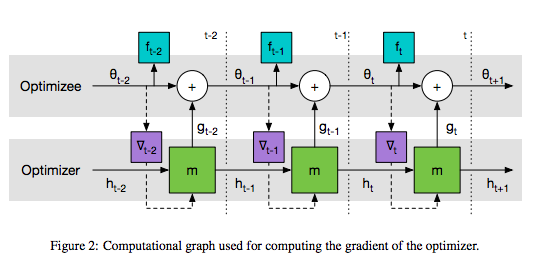
But how do we model the optimizer? We use Recurrent Neural Network. Therefore, the parameters of the oprimizer are just the parameters of RNN. The parameters of the original function in question (i.e. the cost function of “one instance” of a problem that is drawn from a class of optimization problems) are referred as “optimizee parameters”, and are updated using the output of our optimizer, just as we update parameters using the gradient in SGD. The final optimzee parameters $\theta^*$ will be a function of the optimizer parameters and the function in question. In summary:

$$\theta^* (\phi, f) \text{: the final optimzee parameters}$$

$$\phi \text{: the optimizer parameters}$$

$$ f\text{: the function in question} $$

$$
\theta_{t+1} = \theta_t + g_t(\nabla f(\theta_t), \phi) \text{: the update equation of the optimzee parameters}
$$
where $g_t$ is modeled by RNN. So $\phi$is the parameter of RNN. Because LSTM is better than vanilla RNN in general (citation needed*), the paper uses LSTM. Regular gradient descent algorithms use $g_t(\nabla f(\theta_t), \phi) = -\alpha \nabla f(\theta_t)$.

RNN is a function of the current hidden state $h_t$, the current gradient $\nabla f(\theta_t)$, and the current parameter $\phi$.

The “goodness” of our optimizer can be measured by the expected loss over the distribution of a function $f$, which is

$$ L(\phi) = \mathbb{E}_f [f(\theta^* (\phi, f))] $$

(I’m ignoring $w_t$ in the above expression of $L(\phi)$ because in the paper they set $w_t = 1$.)

For example, suppose we have a function like $f(\theta) = a \theta^2 + b\theta + c$. If $a,b,c$ are drawn from the Gaussian distribution with some fixed value of $\mu$ and $\sigma$, the distribution of the function $f$ can be defined. (Here, the class of optimization problem is a function where $a,b,c$ are drawn from Gaussian.) In this example, the optimzee parameter is $\theta$. The optimizer (i.e. RNN) will be trained by optimizing functions which are randomly drawn from the function distribution, and we want to find the best parameter $\theta$. If we want to know how good our optimizer is, we can just take the expected value of $f$ to evaluate the goodness, and use gradient descent to optimize this $L(\phi)$.

After understanding the above basics, all that is left is some implementation/architecture details for computational efficieny and learning capability.

(By the way, there is a typo in page 3 under Equation 3; $\nabla_{\theta} h(\theta)$ should be $\nabla_{\theta} f(\theta)$. Otherwise it doesn’t make sense.)

Coordinatewise LSTM optimizer

[The Figure is from the paper : Figure 2 on page 4]

To make the learning problem computationally tractable, we update the optimzee parameters $\theta$ coordinatewise, much like other successful optimization methods such as Adam, RMSprop, and AdaGrad.

To this end, we create $n$ LSTM cells, where $n$ is the number of dimensions of the parameter of the objective function. We setup the architecture so that the parameters for LSTM cells are shared, but each has a different hidden state. This can be achieved by the code below:

1
2
3

lstm = tf.nn.rnn_cell.BasicLSTMCell(hidden_size)
for i in range(number_of_coordinates):
    cell_list[i] = tf.nn.rnn_cell.MultiRNNCell([lstm_cell] * num_layers) # num_layers = 2 according to the paper.

Information sharing between coordinates

The coordinatewise architecture above treats each dimension independently, which ignore the effect of the correlations between coordinates. To address this issue, the paper introduces more sophisticated methods. The following two models allow different LSTM cells to communicate each other.

1. Global averaging cells: a subset of cells are used to take the average and outputs that value for each cell.
2. NTM-BFGS optimizer: More sophisticated version of 1., with the external memory that is shared between coordinates.

Implementation Notes

Quadratic function (3.1 in the paper)

Let’s say the objective funtion is $f(\theta) = || W \theta - y ||^2$, where the elements of $W$ and $y$ are drawn from the Gaussian distribution.

$g$ (as in $\theta_{t+1} = \theta_t + g$) has to be the same size as the parameter size. So, it will be something like:

1

g, state = lstm(input_t, hidden_state) # here, input_t is the gradient of a hidden state at time t w.r.t. the hidden

And the update equation will be:

1

param = param + g

The objective function is:
$$L(\phi) = \mathbb{E}_f [ \sum_{t=1}^T w_t f(\theta_t) ]$$
$$\text{where, }\theta_{t+1} = \theta_t + g_t$$
$$\left[ \begin{array}{c} g_t \\ h_{t+1} \end{array} \right] = RNN(\nabla_t, h_t, \phi)$$

The loss $L(\phi)$ can be computed by double-for loop. For each loop, a different function is randomly sampled from a distribution of $f$. Then, $\theta_t$ will be computed by the above update equation. So, overall, what we need to implement is the two-layer coordinate-wise LSTM cell. The actual implementation is here.

Results

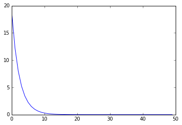
I compared the result with SGD, but SGD tends to work better than our optimizer for now. Need more improvements on the optimization…

Notes on Induced Matrix Norm. I think the name comes from that fact that it is “induced” by a vector.

Definition:
For a $m$ by $n$ matrix $A$, and a n-dimensional vector $x$,
$$|| A ||_p = \sup \{ ||Ax||_p : ||x||_p = 1\}$$

Note that since given $A$, $ ||Ax||_p$ is a function of $x$, which is closed and bounded as $||x||_p = 1$, $||Ax||_p$ achieves maximum or minimum on some $x$. So we can replace $\sup$ with $\max$.

Claim I : $p = 1$:
$$||A||_1 = \max_{1 \le j \le n} \sum_{i=1}^m a_{ij}$$

First, let us find some upper bound on $||Ax||_1$.
$$||Ax||_1 = || \sum_{i=1}^n A_i x_i ||_1 \le \sum_{i=1}^n |x_i| || A_i ||_1 \le \max_j ||A_j|| \sum_{i=1}^n |x_i| = \max_j ||A_j|| ||x||_1$$

So given A, we have found a constant $K = \max_j ||A_j||$ that will upper bound $||Ax||_1$ by $K||x||_1$:
$$||Ax||_1 \le K ||x||_1$$

Next, we show that there exists $x$ for which we have equality for the above equation. Since $K = \max_j ||A_j||$, we can just let $x = [0, 0, …, 1, .. 0, 0]$ where 1 is at the $k$th position. $k$ is the index that satisfies $||A_k|| = \max_j ||A_j||$.

So we’ve found that ||A||_1 = \max_j ||A_j|| .

Claim II : $p = \infty$:
$$||A||_{\infty} = \max_{1 \le i \le m} \sum_{j=1}^n a_{ij}$$

First, consider $|| Ax ||_{\infty}$. Then,

So given $A$, we have found a constant $K = \max_i \left( \sum_{j=1}^n \left | a_{ij} \right | \right)$ that will upper bound $||Ax||_{\infty}$:
$$\| Ax \|_{\infty} \le K  \| x \|_{\infty}$$

To find $\| A \|_{\infty}$, we need to find some $x$ that equates the above inequality, which is fortunately straightforward as in the case of $p = 1$. By examining :

we notice that we achieve the equality if we let
$$x_k = \begin{cases} \frac{ a_{ik} }{ | a_{ik} |} & (a_{ik} \neq 0) \\ 1 & (a_{ik} = 0) \end{cases}$$

where $k$ is the index such that $A_{k,:} = \max_i \left( \sum_{j=1}^n \left | a_{ij} \right | \right)$ Note: I’m using $A_k$ as denoting the $k$ th column vector of a matrix $A$, and $A_{k, :}$ as denoting the $k$ th row vector of $A$.

Claim III : $p = 2$:
$$\|A\|_2 = \sqrt{ \lambda_{\max} }$$
where $\lambda_{\max}$ is the largest eigenvalue of $A^T A$.

This is the spectral norm!

Reference

• https://en.wikipedia.org/wiki/Matrix_norm
• http://www.ece.uah.edu/courses/ee448/chapter4.pdf

Welcome to Hexo! This is your very first post. Check documentation for more info. If you get any problems when using Hexo, you can find the answer in troubleshooting or you can ask me on GitHub.

Quick Start

Create a new post

1

$ hexo new "My New Post"

More info: Writing

Run server

1

$ hexo server

More info: Server

Generate static files

1

$ hexo generate

More info: Generating

Deploy to remote sites

1

$ hexo deploy

More info: Deployment

I decided to do all the practice problems in Chapter 5 of Pattern Recognition and Machine Learning by Bishop. This chapter is about neural nets. Although the material per se is a little bit old, all the fundamentals of neural network are very well explained in here, so even today, when a bunch of new papers on deep neural network come out on arxiv almost everyday, it’s worth reading in my opinion.

So today I did 5.25. The problem reads:

Consider a quadratic error function of the form $ E = E_0 + (w - w^{\ast} )^T H (w - w^{\ast}) $, where $w^{\ast}$ represents the minimum, and the Hessian matrix $H$ is positive definite and constant. Suppose the initial weight vector $w^{(0)}$ is chosen to be at the origin and is updated using simple gradient descent
$$
w^{(\tau)} = w^{(\tau−1)} − \rho \nabla E
$$
where $\tau$ denotes the step number, and $\rho$ is the learning rate (which is assumed to be small). Show that, after $\tau$ steps, the components of the weight vector parallel to the eigenvectors of $H$ can be written
$$
w_j^{(\tau)} = (1 − (1 − \rho \lambda_j )^{\tau} ) w_j^{\ast}
$$
where $w_j = w^Tu_j$ , and $u_j$ and $\lambda_j$ are the eigenvectors and eigenvalues, respectively, of $H$. Show that as $\tau \rightarrow \infty$, this gives $w^{(\tau)} \rightarrow w^*$ as expected, provided $|1 − \rho \lambda_j | < 1$.

I’m assuming that since $H$ is a constant, it is evaluated at $w^{\ast}$, and $E_0 = E(w^{\ast})$.

First, since $H$ is a symmetric matrix, we can say that the eigenvalues are all real, and the eigenvectors are orthogonal to each other.

WLOG, we assume the $u_i$s are orthonormal. So the $u_i$s form the orthonormal basis, meaning we can express any vector with these basis vectors. This means that we can express $w - w^{\ast} = \sum_i^n v_i u_i$, where $v_i$s are appropriate coefficients. We can rewrite the equation using matrix form, which is $w - w^{\ast} = U v \iff v = U^T (w - w^{\ast})$, where $U$’s columns are $u_i$s. This expression gives us new perspective: we can view the weight vector $w$ in the original coordinate with a different coordinate, which is obtained by moving $w^{\ast}$ to the origin and rotate the original coordinate by the rotation matrix $U$.

Let’s plug this into the given error function E. We get
$$
E = E_0 + \frac{1}{2} (Uv)^T H (Uv) = E_0 +\frac{1}{2} v^T U^T H U v
$$

Note that $H$ is a symmetric, meaning it is diagonalizable. So we get
$$
E = E_0 + \frac{1}{2} v^T U^T UDU^T U v
$$

Since U is an orthonormal matrix, we have this identity $U^T = U^{-1}$ so everything cancels out, yielding $E = E_0 + \frac{1}{2} v^T D v$.

Note that $E$ is a function of $w$: $E(w)$. What if we look at it from the new coordinate? We see that $E_0(w^{\ast})$ should be 0 because in the new coordinate $w^{\ast}$ is the origin. Then, we have
$$
E(v) = \frac{1}{2} v^T D v = \frac{1}{2} \sum_i^n \lambda_i v_i^2
$$
(Note that D is a diagonal matrix with diagonal elements being eigenvalues.)

Then,
$$
\nabla E_v(v) = D v = \sum_i^n \lambda_i v_i
$$
So, the update equation becomes
$$
v^{(\tau)} = v^{(\tau-1)} - \rho D v^{(\tau-1)} = (I - \rho D) v^{(\tau - 1)}
$$

If we look at the last equation coordinate wise, we get $v_i^{(\tau)} = (1 - \rho \lambda_i) v_i^{(\tau - 1)} $, so by recursion, we get
$$
v_i^{(\tau)} = (1 - \rho \lambda_i)^{\tau} v_i^{(0)}
$$
Now, let’s go back to the original coordinate, and we get
$$
w_i^{(\tau)} - w_i^{\ast} = (1 - \rho \lambda_i)^{\tau} w_i^{(0)} - w_i^{\ast}
$$
Since w^{(0)} is the origin, the left term is 0 and moving $w_i^{\ast}$ to left, we get
$$
w_i^{(\tau)} = (1 - (1 - \rho \lambda_i)^{\tau})w_i^{\ast}
$$
, which is what we wanted to show.

LU decomposition

Thm 1:
N-rank regular matrix A has a unique factorization LU, where L is a N-rank regular matrix and U is a N-rank upper-triangular matrix.

When we think about the signs of eigenvalues in neural network literature, we only deal with Hessian, which is symmetric, so the signs of all eigenvalues uniquely determine the positive definiteness of the Hessian matrix. But this is not generally true for non-symmetric positive definite matrix.

One example of equivalent condition of a matrix being positive definite is the existence of a unique lower triangular matrix L with real and strictly positive diagonal entries s.t. M = LL holds. (M = LL is called Cholesky decomposition.)

Cholesky decomposition

Thm 2:
For a symmetric positive definite matrix M, there exists a decomposition s.t. M = LL^T

Pf. (sketch)
$$M = PDP^T \\ = PSS^TP^T \\ = B^TB \quad (B = (PS)^T) \\ = (QR)^T QR \quad (B = QR) \\ = R^T Q^{-1} Q R = R^T R = LL^T$$

Compute Hessian using TensorFlow

Reference:

• TensorFlow implementation of K-means algorithm: https://codesachin.wordpress.com/2015/11/14/k-means-clustering-with-tensorflow/
• Calculating Hessian in Theano (application for Newton’s method): https://groups.google.com/forum/#!topic/theano-users/2c15kq68lp8

TensorFlow has a function called tf.gradients() that computes gradient. In the past, I’ve tried to compute Hessian of an neural network objective function in Torch7 using torch-autograd but it was somewhat cumbersome; there wasn’t an easy way to store/reshape parameters because Lua uses table for everything. Today, I’d like to do the same thing in TensorFlow. It should be much easier than in Torch7 due to the symbolic differentiation.

Example 1 : Quadratic function

We are going to use $f(x) = \frac{1}{2} x^T A x + b^T x + c$ as our first example to compute Hessian. When A is a symmetric matrix, the hessian of $f$ should be equal to $A$.

For simplicity, let us start with:
$$A = \left[ \begin{array}{rrr} 2 & 2 & 2 \\ 2 & 2 & 2 \\ 2 & 2 & 2 \end{array} \right] \quad b = \left[ \begin{array}{rrr} 3 \\ 3 \\ 3 \end{array} \right] \quad c = 1$$

The code below calculates the hessian for f(x).

1
2
3
4

import tensorflow as tf
import matplotlib as plt
import numpy as np
import math

1
2
3
4
5
6
7
8
9
10
11
12
13
14
15
16
17
18
19
20
21
22
23
24
25
26
27
28
29
30
31
32
33
34
35
36
37
38
39

def getHessian(dim):
    # Each time getHessian is called, we create a new graph so that the default graph (which exists a priori) won't be filled with old ops.
    g = tf.Graph()
    with g.as_default():
        # First create placeholders for inputs: A, b, and c.
        A = tf.placeholder(tf.float32, shape=[dim, dim])
        b = tf.placeholder(tf.float32, shape=[dim, 1])
        c = tf.placeholder(tf.float32, shape=[1])
        # Define our variable
        x = tf.Variable(np.float32(np.repeat(1,dim).reshape(dim,1)))
        # Construct the computational graph for quadratic function: f(x) = 1/2 * x^t A x + b^t x + c
        fx = 0.5 * tf.matmul(tf.matmul(tf.transpose(x), A), x) + tf.matmul(tf.transpose(b), x) + c
        
        # Get gradients of fx with repect to x
        dfx = tf.gradients(fx, x)[0]
        # Compute hessian
        for i in range(dim):
            # Take the i th value of the gradient vector dfx 
            # tf.slice: https://www.tensorflow.org/versions/0.6.0/api_docs/python/array_ops.html#slice
            dfx_i = tf.slice(dfx, begin=[i,0] , size=[1,1])
            # Feed it to tf.gradients to compute the second derivative. 
            # Since x is a vector and dfx_i is a scalar, this will return a vector : [d(dfx_i) / dx_i , ... , d(dfx_n) / dx_n]
            ddfx_i = tf.gradients(dfx_i, x)[0] # whenever we use tf.gradients, make sure you get the actual tensors by putting [0] at the end
            if i == 0: hess = ddfx_i
            else: hess = tf.concat(1, [hess, ddfx_i]) 
            ## Instead of doing this, you can just append each element to a list, and then do tf.pack(list_object) to get the hessian matrix too.
            ## I'll use this alternative in the second example.  
        # Before we execute the graph, we need to initialize all the variables we defined
        init_op = tf.initialize_all_variables()
    
        with tf.Session() as sess:
            sess.run(init_op)
            # We need to feed actual values into the computational graph that we created above. 
            feed_dict = {A: np.float32(np.repeat(2,dim*dim).reshape(dim,dim)), b: np.float32(np.repeat(3,dim).reshape(dim,1)) , c: [1]}
            # sess.run() executes the graph. Here, "hess" will be calculated with the values in "feed_dict".
            print(sess.run(hess, feed_dict))

1

getHessian(3)

[[ 2.  2.  2.]
 [ 2.  2.  2.]
 [ 2.  2.  2.]]

We can see that the result of sess.run(hess, feed_dict) is indeed the desired value: A

Example 2 : Multilayer Perceptron

Next, we’ll try a small neural network model: Multilayer perceptron. We need to modify our getHessian function a little bit; we need to create one-long vector for parameters, and then slice them according to the model architecture. Otherwise tf.gradients() cannot calculate the hessian matrix.

1
2
3
4
5
6
7
8
9
10
11
12
13
14
15
16
17
18
19
20
21
22
23
24
25
26
27
28
29
30
31
32
33
34
35
36
37
38
39
40
41
42
43
44
45
46
47
48
49
50
51
52
53

def getHessianMLP(n_input, n_hidden, n_output):
    batch_size = 1
    # Each time getHessianMLP is called, we create a new graph so that the default graph (which exists a priori) won't be filled with old ops.
    g = tf.Graph()
    with g.as_default():
        # First create placeholders for inputs and targets: x_input, y_target
        x_input = tf.placeholder(tf.float32, shape=[batch_size, n_input])
        y_target = tf.placeholder(tf.float32, shape=[batch_size, n_output])
    
        # Start constructing a computational graph for multilayer perceptron
        ###  Since we want to store parameters as one long vector, we first define our parameters as below and then
        ### reshape it later according to each layer specification.
        parameters = tf.Variable(tf.concat(0, [tf.truncated_normal([n_input * n_hidden, 1]), tf.zeros([n_hidden, 1]),
                                                                                                      tf.truncated_normal([n_hidden * n_output,1]), tf.zeros([n_output, 1])]))
        
        with tf.name_scope("hidden") as scope:
            idx_from = 0 
            weights = tf.reshape(tf.slice(parameters, begin=[idx_from, 0], size=[n_input*n_hidden, 1]), [n_input, n_hidden])
            idx_from = idx_from + n_input*n_hidden
            biases = tf.reshape(tf.slice(parameters, begin=[idx_from, 0], size=[n_hidden, 1]), [n_hidden]) # tf.Variable(tf.truncated_normal([n_hidden]))
            hidden = tf.matmul(x_input, weights) + biases
        with tf.name_scope("linear") as scope:
            idx_from = idx_from + n_hidden
            weights = tf.reshape(tf.slice(parameters, begin=[idx_from, 0], size=[n_hidden*n_output, 1]), [n_hidden, n_output])
            idx_from = idx_from + n_hidden*n_output
            biases = tf.reshape(tf.slice(parameters, begin=[idx_from, 0], size=[n_output, 1]), [n_output]) 
            output = tf.nn.softmax(tf.matmul(hidden, weights) + biases)
        # Define cross entropy loss
        loss = -tf.reduce_sum(y_target * tf.log(output))
        
        
        ### Note: We can call tf.trainable_variables to get GraphKeys.TRAINABLE_VARIABLES 
        ### because we are using g as our default graph inside the "with" scope. 
        # Get trainable variables
        tvars = tf.trainable_variables()
        # Get gradients of loss with repect to parameters
        dloss_dw = tf.gradients(loss, tvars)[0]
        dim, _ = dloss_dw.get_shape()
        hess = []
        for i in range(dim):
            # tf.slice: https://www.tensorflow.org/versions/0.6.0/api_docs/python/array_ops.html#slice
            dfx_i = tf.slice(dloss_dw, begin=[i,0] , size=[1,1])
            ddfx_i = tf.gradients(dfx_i, parameters)[0] # whenever we use tf.gradients, make sure you get the actual tensors by putting [0] at the end
            hess.append(ddfx_i)
        hess = tf.squeeze(hess) 
        init_op = tf.initialize_all_variables()
        with tf.Session() as sess:
            sess.run(init_op)
            feed_dict = {x_input: np.random.random([batch_size, n_input]), y_target: np.random.random([batch_size, n_output])}
            #print(sess.run(loss, feed_dict))
            print(hess.get_shape())
            print(sess.run(hess, feed_dict))

1

getHessianMLP(n_input=3,n_hidden=4,n_output=3)

(31, 31)
[[  2.19931314e-03  -1.42659002e-03   1.30957202e-03  -8.70158256e-04
    8.50890204e-03  -5.51932165e-03   5.06659178e-03  -3.36654740e-03
    7.25943921e-03  -4.70885402e-03   4.32260381e-03  -2.87219742e-03
    1.87662840e-02  -1.21727986e-02   1.11743081e-02  -7.42488075e-03
   -5.90046346e-02   8.59218910e-02  -2.69172415e-02  -1.75508182e-03
    3.87416431e-03  -2.11908249e-03  -5.98554593e-03   1.32124824e-02
   -7.22693698e-03   3.56099289e-03  -7.86052924e-03   4.29953635e-03
   -1.33406427e-02   2.94481106e-02  -1.61074679e-02]
 [ -1.42659002e-03   2.15499196e-03   2.23391340e-03   5.85207134e-04
   -5.51932165e-03   8.33742879e-03   8.64276756e-03   2.26410269e-03
   -4.70885402e-03   7.11314566e-03   7.37364776e-03   1.93163764e-03
   -1.21727986e-02   1.83881018e-02   1.90615226e-02   4.99345176e-03
   -2.40529864e-03  -1.63234770e-02   1.87287778e-02  -5.11422716e-02
    6.40287027e-02  -1.28864162e-02  -1.72071008e-03  -1.16775408e-02
    1.33982506e-02   1.02370558e-03   6.94734277e-03  -7.97104836e-03
   -3.83513537e-03  -2.60270163e-02   2.98621524e-02] ... [omitted] ]