Metric Learning Part1
Metric Learning: Part 1
Note: this post is the first part of the distance metric series. The first post discusses “Distance Metric Learning, with application
to clustering with side-information” (http://ai.stanford.edu/~ang/papers/nips02-metric.pdf) and the
second post discusses “Geometric Mean Metric Learning” (http://suvrit.de/papers/GMML.pdf)
I attended one of the optimization session on the first day of ICML and one of the talks I listened to was about geometric
mean metric learning (http://suvrit.de/papers/GMML.pdf). I was amazed by their result so I’ll make some notes about
their method for myself.
In many machine learning tasks (i.e. classification, search, clustering),
it is necessary to learn some sort of notion of distance between input
data points. For example, in classification, one needs to –
Metric learning was (first?) introduced in this paper: “Distance Metric Learning, with application
to clustering with side-information”
http://ai.stanford.edu/~ang/papers/nips02-metric.pdf.
Problem Setting
Suppose we have a set of points $\{x_i\}_{i=1}^n \subseteq R^m$. Suppose also we are given a set of “side information” that tells us that a certain set of points are “similar” s.t. $S: (x_i, x_j) \in S \text{ if } x_i \text{ and } x_j \text{ are similar. }$ How can we encode this similar-dissimilar information in a distance metric?
Simple answer
Learn a Mahalanobis distance $d(x,y) = \sqrt{(x-y)^T A (x-y)}$ so that $A$ will somehow encode the desired information.
Now the problem is reduced to how to learn the matrix A. Whenever we want to learn something, we should remind ourselves of viewing it as optimization. To do so, we need to define what we want to minimize (or maximize…just flip the sign of the objective function), which should correspond to the notion of “goodness” of the matrix A. But before that, we will go over how the Mahalanobis distance came in.
Mahalanobis distance in R^2
To get the feel of it, we will look at some examples.
|
|
|
|

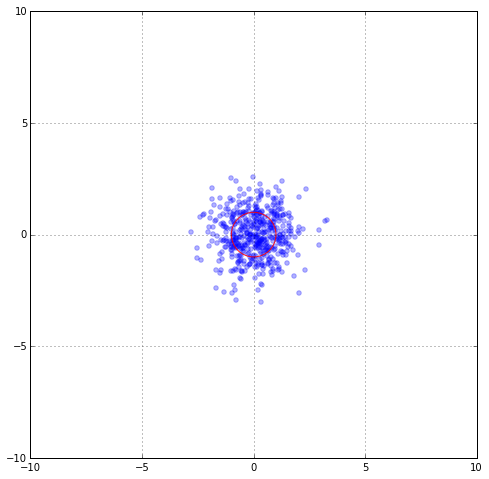
Suppose that the data distribution were Gaussian and our data samples are distributed according to $N(0, I)$. The red circle marks the unit standard deviation. Now, take two blue points x and y. The Euclidian distance between x and y is $|| x - y ||_2 = \sqrt{(x-y)^T (x-y)}$. Now normally the data are not distributed according to Gaussian, but rather some obscure distribution. In this data distribution, some data samples might be “similar” and others are not. If we use Euclidian distance as a way to measure similarity, we might end up disregarding the intrinsic information within the data distribution. We want to “correct” this.
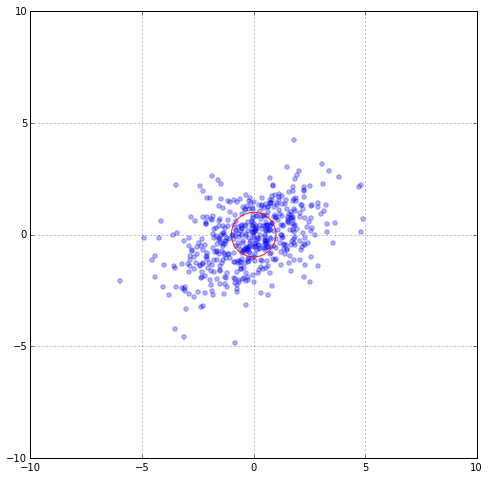
To be more concrete, suppose our real data distribution were something like $\mu = 0$ and $Cov = [[1,0], [0, 6]], which is still too simplistic for any real data. Then sample distribution might look like this:
|
|

In order to reflect the distortion, we should use ; what is the correct way to measure the distance between x and y in the new plot? For example, can we say that the point at the top of the distribution and that point right this and this are the same distance? We should fix this because we think that those two points that are along the principle direction should be “more” similar than those that are not (in this case perpendicular). How can we fix this? By rotating back. The rotation matrix we used was C. So one correct distance metric we could use is $|| x - y ||_{C^{-1}} = \sqrt{(x-y)^T C^{-1} (x-y)}$
Now let’s go back to the paper. What the paper says is this: why not let the data decide which matrix $C^{-1}$ to use.
Optimization problem
The simplest formulation would be : $\min \sum_{x_i, y_i \in S} || x_i - y_i ||_A$. However, this would lead to the non-interesting answer which is to let A be 0 matrix, which will give us 0 for even pairs of x and y which are in a dissimilar set $D$. So we should have a restriction which prevents that to happen. One way to do is add a constraint on $A$ such that $\sum_{x_i, y_i \in D} || x_i - y_i ||_A \ge c$, where $c$ is some positive constant. such that (most of) $|| x_i - y_i ||_A = 0$ even if $x_i \neq y_i$, which is not even a distance anymore. (Recall the definition of “distance”.) So the final form is:
$\min \sum_{x_i, y_i \in S} || x_i - y_i ||_A \text{ s.t. } \sum_{x_i, y_i \in D} || x_i - y_i ||_A \ge c \text{ and } A \succeq 0$